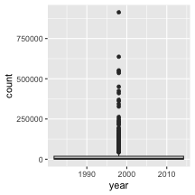
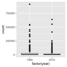
class: center, middle, inverse, title-slide .title[ # Stat 579: Missing values and Factor variables ] .author[ ### Heike Hofmann ] --- # Missing values - missing values in R are encoded as `NA` (for Not Available) - missing values are 'contagious': ```r 1 + NA ``` ``` ## [1] NA ``` ```r max(c(1, 2, 3, NA)) ``` ``` ## [1] NA ``` ```r mean(c(1, 2, 3, NA)) ``` ``` ## [1] NA ``` ```r x == NA ``` ``` ## [1] NA ``` --- # Missing values (2) - Check for missing values with `is.na` ```r is.na(c(1, 2, 3, NA)) ``` ``` ## [1] FALSE FALSE FALSE TRUE ``` - address missing values specifically and systematically: a lot of functions have argument `na.rm` (remove `NA`) ```r mean(c(7, 4, NA, 10), na.rm=TRUE) ``` ``` ## [1] 7 ``` ```r cor(c(7, 4, NA, 10), c(1,2,3,4), use = "pairwise.complete") ``` ``` ## [1] 0.6546537 ``` --- # Missing values (3) - Note: `NA` is different from `NaN` (not a number) and `Inf`: ```r 1/0 ``` ``` ## [1] Inf ``` ```r 0/0 ``` ``` ## [1] NaN ``` - missing values come last (by default), ```r order(c(7, 4, NA, 10)) ``` ``` ## [1] 2 1 4 3 ``` - **careful:** `sort` quietly drops `NA` values ```r length(sort(c(7, 4, NA, 10))) ``` ``` ## [1] 3 ``` --- # Dealing with missing values A lot of functions deal with getting rid of missing values: `?na.omit`, `?complete.cases` It is dangerous and usually results in wrong conclusions to simply reduce a data set to complete records only. Values can be missing for a variety of reasons: (completely) at random or according to some mechanism involving other variables Example (homework file) ```r iowa <- read.csv("https://raw.githubusercontent.com/Stat579-at-ISU/stat579-at-isu.github.io/master/homework/data/brfss-iowa-2022.csv") dim(iowa) ``` ``` ## [1] 8949 326 ``` ```r sum(complete.cases(iowa)) ``` ``` ## [1] 0 ``` --- class: inverse # Your Turn - Inspect the `fbi` object. - Which variable(s) have missing values? how many? - Create a subset of the fbi that contains all missing values. Can you identify a pattern in the structure of missing values? --- ``` missing %>% ggplot(aes(x = year, y = state_abbr)) + geom_tile() missing %>% ggplot(aes(x = year, y = type)) + geom_tile() ``` --- class: inverse, center, middle # Factors --- # Factors - A special type of variable to indicate categories - both *labels* and their *order* (i.e. numbers) - By default text variables are stored in factors during input - numeric categorical variables have to be converted to factors manually - `factor` creates a new factor with specified labels --- class: inverse # Your Turn - Inspect the `fbi` object. How many variables are there? Which type does each of the variables have? - Make a summary of Year - Make Year a factor variable: `fbi$year <- factor(fbi$year)` - Compare summary of Year to the previous result - Are there other variables that should be factors (or vice versa)? --- # Note: factors in boxplots boxplots in ggplot2 only work properly if the x variable is a character variable or a factor: ```r twoyear <- dplyr::filter(fbi, year %in% c(1980, 2016)) ``` .pull-left[ ```r ggplot(data = twoyear, aes(x = year, y = count)) + geom_boxplot() ``` <!-- --> ] .pull-right[ ```r ggplot(data = twoyear, aes(x = factor(year), y = count)) + geom_boxplot() ``` <!-- --> ] --- # Data types: checking and casting Checking for, and casting between types: - `str`, `mode` provide info on type - `is.XXX` (with XXX either `factor, int, numeric, logical, character, ...` ) checks for specific type - `as.XXX` casts to specific type --- # Casting between types  **Note:** `as.numeric` applied to a factor retrieves *order* of labels, not labels, even if those could be interpreted as numbers. To get the labels of a factor as numbers, first cast to character and then to a number. --- # Levels of factor variables - `levels(x)` shows us the levels of factor variable `x` in their current order - factor variables often have to be re-ordered for ease of comparisons - We can specify the order of the levels by explicitly listing them, see `help(factor)` - We can make the order of the levels in one variable dependent on the summary statistic of another variable --- # Reordering factor levels - manual ```r fbi$type <- factor(fbi$type) levels(fbi$type) ``` ``` ## [1] "aggravated_assault" "arson" "burglary" ## [4] "homicide" "larceny" "motor_vehicle_theft" ## [7] "rape_legacy" "rape_revised" "robbery" ``` manually (extremely sensitive to typos): ```r levels(factor(fbi$type, levels=c("larceny", "burglary", "motor_vehicle_theft", "aggravated_assult", "robbery", "rape_legacy", "homicide", "rape_revised"))) ``` ``` ## [1] "larceny" "burglary" "motor_vehicle_theft" ## [4] "aggravated_assult" "robbery" "rape_legacy" ## [7] "homicide" "rape_revised" ``` --- # The `forcats` package - part of the tidyverse set of packages - goal: make working with factors easier - Four main functions: - `fct_reorder()`: Reordering a factor by another variable. - `fct_infreq()`: Reordering a factor by the frequency of values. - `fct_relevel()`: Changing the order of a factor by hand. - `fct_lump()`: Collapsing the least/most frequent values of a factor into "other". --- # Reordering factor levels - using another variable `reorder(factor, numbers, function)` reorder levels in factor by values in `numbers`. Use `function` to summarise (average is used by default). ```r levels(reorder(fbi$type, fbi$count, na.rm=TRUE)) ``` ``` ## [1] "homicide" "arson" "rape_legacy" ## [4] "rape_revised" "robbery" "aggravated_assault" ## [7] "motor_vehicle_theft" "burglary" "larceny" ``` missing values in `numbers`? make sure to use parameter `na.rm=TRUE`! --- class: inverse ## Your turn For this your turn use the `fbi` object from the `classdata` package. - Introduce a rate of the number of reported offenses by population into the `fbi` data. You could use the *Ames standard* to make values comparable to a city of the size of Ames and Story county (population ~100,000). - Plot boxplots of crime rates by different types of crime. How can you make axis text legible? - Reorder the boxplots of crime rates, such that the boxplots are ordered by their medians. - For one type of crime (subset!) plot boxplots of rates by state, reorder boxplots by median crime rates --- # Changing Levels' names ```r levels(fbi$type) ``` ``` ## [1] "aggravated_assault" "arson" "burglary" ## [4] "homicide" "larceny" "motor_vehicle_theft" ## [7] "rape_legacy" "rape_revised" "robbery" ``` ```r levels(fbi$type)[4] <- "murder" levels(fbi$type) ``` ``` ## [1] "aggravated_assault" "arson" "burglary" ## [4] "murder" "larceny" "motor_vehicle_theft" ## [7] "rape_legacy" "rape_revised" "robbery" ``` --- # Read more on factors - Wickham & Grolemund's <a href="http://r4ds.had.co.nz/factors.html">chapter on factors</a> in *R for Data Science* - Roger Peng: [*stringsAsFactors: An unauthorized biography*](http://simplystatistics.org/2015/07/24/stringsasfactors-an-unauthorized-biography/") - Thomas Lumley: <a href="http://notstatschat.tumblr.com/post/124987394001/stringsasfactors-sigh"><em>stringsAsFactors = &lt;sigh&gt;</em></a> - The <a href="https://forcats.tidyverse.org/">`forcats` package</a> has a lot of additional functions that make working with factors easier.